
We are ultimately concerned with developing positive dynamic models of commerce on a growing social network, from network inception to large scale adoption.
Of course our initial efforts simplify the problem in various ways. One way is to limit our focus to static networks with varying network characteristics. Simulating dynamically changing networks will come later.
In other ways, the economic model presented here is a vastly simplified model of reality, yet it does possess a rich set of governing parameters and mechanisms that require methodical study. Already the model exhibits complex behavior. Through parametric simulation we are laying a foundation of understanding that we will grow from.
With this in mind this article will describe in detail our first economic model and associated approach to simulation. We also include an example simulation showing inputs and outputs.
Network
In this world we envision a small number of people banding together to form a community (Polis) and to start to interact economically and otherwise. Eventually these small communities will start to connect with other similar communities and in doing so increase the footprint of the overall network.
Considering this, our initial modeling employs static, undirected networks consisting of ~100 agents, or a medium sized singular community. They are undirected because we assume trust is always mutual (not one way).
The networks used in our modeling are randomly created using the preferential attachment model as described here. These synthetic networks exhibit power law scaling found in many social and economic real world networks making them suitable for our study.
Money
Every member of a community will receive a universal basic income (UBI) issued in their own personal currency. The provision of UBI is motivated to provide a minimum level of subsistence to Polis members and allows them to use this money to buy goods and services from network members.
The modeling parameters are 1) the initial award at the start of the simulation, which can be zero, 2) the amount awarded per award interval and 3) the award interval in time. Currently these variables are constant and do not vary during a simulation.
Example: Agent Zeta joins Polis Alpha and earns zero initial Zeta coins but earns 25 Zeta coins every 4 weeks.
While each agent possesses their own coin type, each coin type possesses the same value. There is no exchange rate between, say, Agent A's coins and Agent B's coins.
Money Exchange
Any agent directly connected to another agent is considered to have a "trust" relationship, meaning they, along with the consensus of all network participants (consensus algorithm), have established that they are who they say they are and therefore trust each other.
Agents who trust each other directly can exchange their coins and they can also exchange coins they might possess from mutually trusted agents.
Example: Agents A, B and C are connected and therefore trust each other. If B buys from C, C is willing to take any combination of A and B coins from B since C trust them both (and C will accept C coins).
Agents on the network that are not direct connections are not trusted connections and can exchange coins only through mutually trusted intermediary agents via a chaining transaction process named transitive-transaction.
The transitive-transaction process is described in detail here.
Example: D is connected to A (above) only. If D wants to buy from C, A needs to act as an intermediary taking D's coins and giving trusted coins to C (some combination of A, B and / or C coins that A possess).
If A does not have enough coins to meet the sales price the transaction fails. We call this the "liquidity situation". A detailed description of the liquidity situation can be found here.
Demurrage
Traditionally demurrage is a term associated with seafaring whereby one is charged a fee if they take too long to load or unload their cargo.
Here it is used as a system wide incentive to spend your UBI whereby non-circulating coins are automatically periodically removed from one's wallet and destroyed. The existence of demurrage also controls the level money supply in the long run via this constant destruction of currency.
The modeling parameters are 1) the percentage (%) of your coin value removed at each interval, applied pro rata across the different coin types one might possess, and 2) the interval in time that demurrage is applied. Currently these variables are constant and do not vary during the simulation.
Example: Agent Zeta's account is reduce in value by 5% every 4 weeks. If agent Zeta has 75 zeta coins and 25 beta coins from agent Beta, then Zeta loses 3.75 zeta coins and 1.25 beta coins.
In any given simulation time step Demurrage is applied before UBI is awarded.
Market Participants
We define market participants as Buyers, Sellers and Non-Participants. All participants are Buyers. All participants can be Sellers.
The modeling parameters are 1) the percentage of agents that are Non-Participants, and 2) the percentage of remaining participants that are Sellers. Note that all remaining participants are Buyers.
In any given simulation the Non-Participants are chosen randomly on the network, then the Sellers are chosen randomly from the remaining participants. These assignments remain fixed throughout the simulation.
Example: We have a network consisting of 100 agents, 5% are deemed Non-Participants, meaning they will not buy or sell (but they do support transitive-transactions). 15% of remaining participants are deemed Sellers and all the remaining participants are Buyers. This results in 5 randomly chosen agents being Non-Participants, 14 randomly chosen participants being Sellers and 95 participants being Buyers.
Goods And Services
This initial model is extremely simple. Each Seller sells the same product at the same price P. We can think of the product as some basket of goods.
The modeling parameters are 1) the price P of the basket of goods and 2) the amount of inventory (units) each Seller possesses at the beginning of the simulation. The price and inventory level specified remain fixed for the entire simulation.
Example: There are 14 Sellers selling the same basket of goods for price = 100. Each Seller starts the simulation with 100 units of inventory.
Transaction Distance On A Network
We assume untrusted agents located far away from each other on the network are not likely to want to do business with each other and so we envision some maximum distance whereby untrusted agents are likely to transact.
Therefore, we define the transaction-distance to be the maximum distance allowed for a transaction to occur between a Buying and Selling agent. In other words, Buyers are only allowed to buy from the Sellers that reside within the transaction-distance.
The transaction-distance is an input parameter to the simulation. It's constant and is applied network wide.
Example: Agent A is connected to Agent B and Agent B is connected to Agent C. C and A then are separated from each other by a distance of 2 (with this simple network having a diameter of 2). If the transaction-distance is 1, then A and C cannot transact with each other, they can only transact with B.
The transaction-distance can have a large effect on the simulation dynamics when it is much less than the diameter of the network being used in the simulation. This is because some Sellers are always going to be excluded from some Buyers. If the transaction-distance is equal to or greater than the network diameter then all Sellers will be available to all Buyers making the transaction-distance irrelevant.
The Simulation Approach
A simulation sets in motion the dynamics of the marketplace. The simulation duration is controlled by the specified number of time steps.
During each time step the following happens:
- If it is time, demurrage and / or UBI is applied to all agents
- The Buyers are randomlly sorted, then one at a time,
- Each Buyer attempts to make a purchase from a Seller.
- The Seller is selected randomly from the pool of available Sellers that reside within the transaction-distance of the Buyer
- The transaction is attempted using the transtive-transaction algorithm
Note, Sellers to not buy from themselves.
If the transaction is successful the monies are transferred and the Sellers inventory is decremented. Failed transactions are also recorded.
There are four ways the transaction can fail:
- No liquid paths were found between the Buyer and Seller (Liquidity Failure)
- No Sellers were found within the Buyers transaction-distance (No Seller Failure)
- The Seller selected was out of inventory (No Inventory Failure)
- The Buyer did not have enough money to meet the purchase price (No Money Failure)
Ultimately we seek situations where commerce happens and money flows. In other words we want Buyers to be able to spend their UBI and for Sellers to sell their products and spend their earnings.
To that end, as a way to compare different simulations, we define a simple measure of commerce that we call "sales efficiency". Sales efficiency is defined to be the ratio of the successfully completed transactions divided by the total possible transactions that could occur in a given simulation.
Example: We have a network of 10 agents, all Buyers (no Passive agents) and 2 Sellers (Buyer / Sellers really). Therefore, in each time step there are 10 possible opportunities to buy (each Buyer tries once). If the simulation duration is 2 time steps then the total possible number of purchases is 20. If for some reason a total of 4 fail, it does not matter in which time step they failed, then the resulting sales efficiency would be (20-4)/20 = 0.8 or 80%.
A Simulation Example
Phew, finally, thanks for getting this far! We'll now show a complete example of a simulation.
The input parameters are:
- The simulation duration is 52 weeks (1 week per time step)
- Since the model possesses a number of random variables we repeat the simulation 16 times and aggregate results
- The price of a basket of goods is 300 Euros
- UBI of 360 Euros is provided weekly (equal to 1,440 Euros annually). Seed UBI is zero.
- Demurrage is 5% applied monthly (~60% annually)
- Sellers have 3000 units of inventory each (essentially infinite inventory)
- The transaction-distance is 3 (so as far as your friends, friends, friends)
- There are 100 agents
- 5% of agents will be passive, randomly selected each iteration
- 10% of agents will be Sellers, randomly selected each iteration
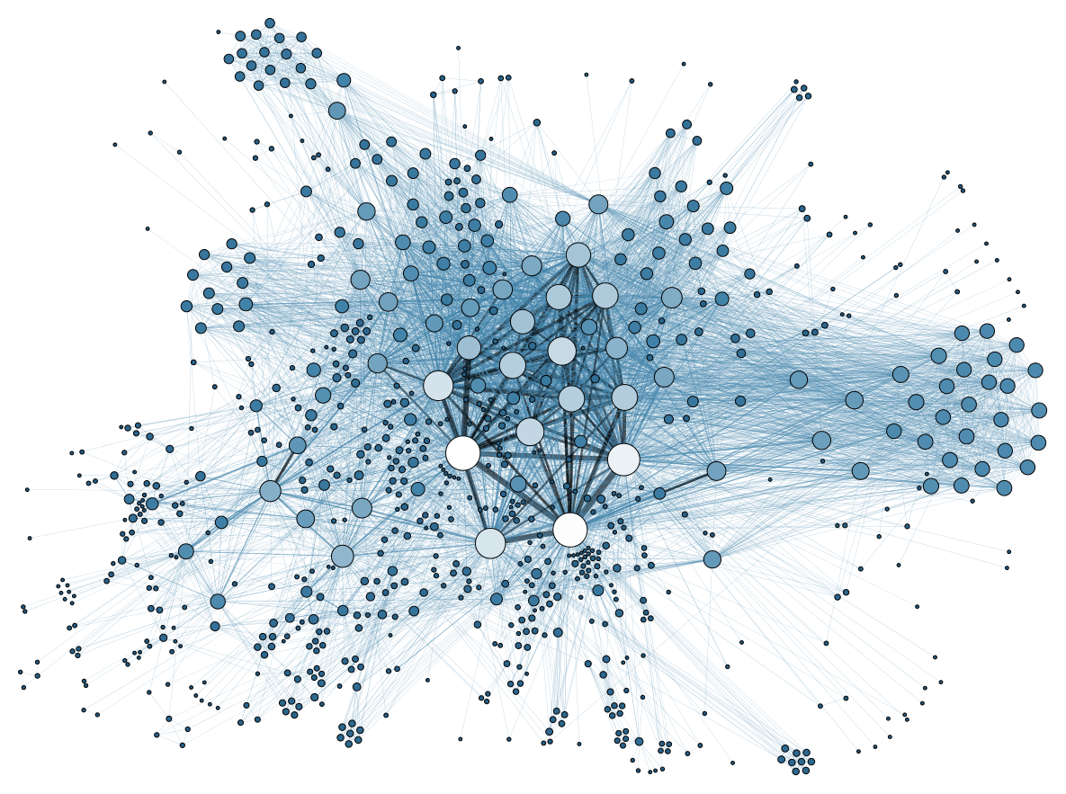
A picture of the network used in this simulation is shown below (Network statistics are provided in the caption). Node size and color is proportional to the number of connections (degree) each agent possesses.
The main results of the simulation are summarized in the table below:
| Measure | Average | Standard Deviation |
|---|---|---|
| Sales Efficiency | 28.78% | 9.94% |
| No Liquidity | 71.08% | 9.80% |
| No Seller | 0.13% | 0.36% |
| No Inventory | 0.0% | 0.0% |
| No Money | 0.0% | 0.0% |
We immediately notice the sales efficiency is less than 30%. We typically seek a realistic set of inputs that result in 90% or better for sales efficiency, so this is quite low. The standard deviation is quite large too showing there is quite a bit of variability from iteration to iteration.
Asking why the sales efficiency is so low we next notice there is a dominating number of liquidity failures and an almost negligible number of no seller failures. So the "liquidity situation" is the problem in this scenario.
We have developed a number of visualization tools to help us understand what happened in more detail. We'll go through those now.
The summary below plots the 100 agents against final individual wallet size, units bought and sold, who were sellers and passive agents and overall money supply.
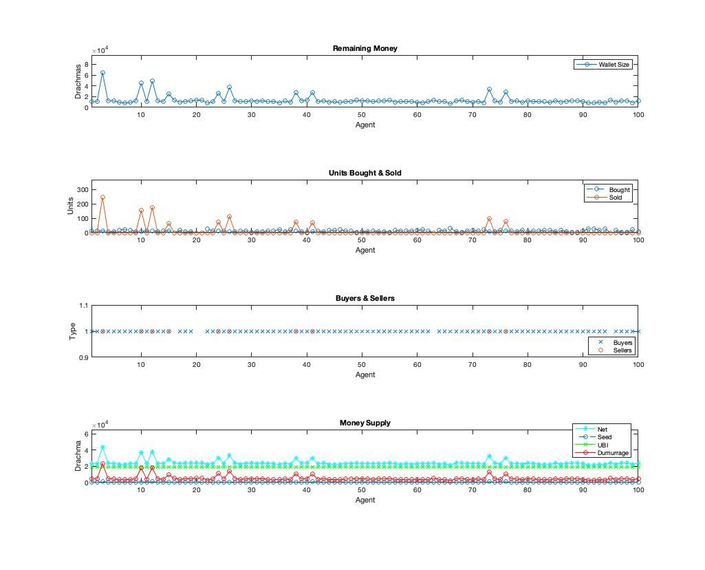
In this diagram it's easy to see the Sellers (Agent 10 for example) are the ones who end up with more money and as a consequence pay the more demurrage.
The next figure (below) plots the total number of deal failures experienced by each agent by type in time.
From this plot we understand that liquidity failures were not transient but are persistent at a fairly constant rate throughout the iteration.
Digging deeper, the figure below shows the number of deal failures by type by agent.
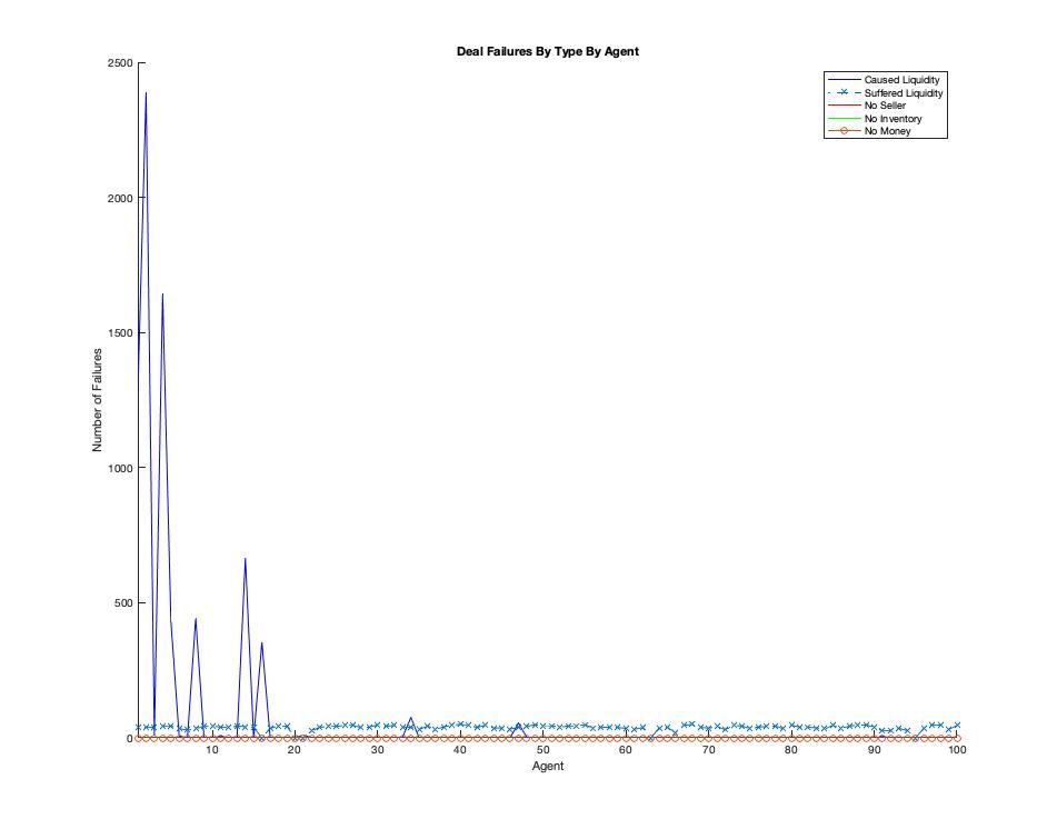
Here we can see that the vast majority of liquidity failures were due to 5 agents, the oldest agents on the network and those that possess the greatest number of connections. So commerce is being forced through these agents as they are the great "connectors" and they do not have the liquidity to do many deals. The liquidity situation strikes again.
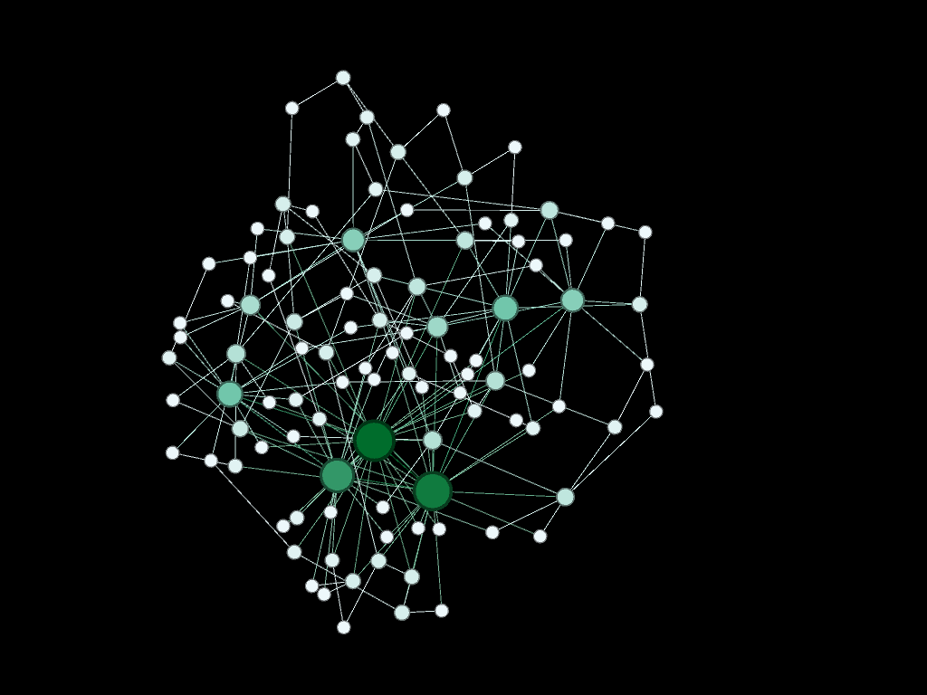
A final look may be had in the network figure below. Here we see the spectrum of liquidity failures across the network. Node size is a function of the degree of the agent (number of connections). The number of liquidity failures are colored in a spectrum from blue (lowest in number) to red (highest in number).
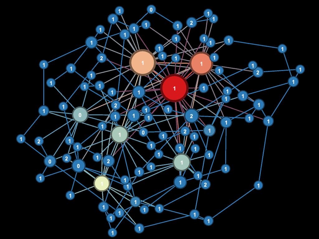
Again we see the nodes with the most connections caused the majority of the liquidity failures as paired Buyers and Sellers are connected through them. We can glean a little more if we note that nodes marked 0 are Passive agents, 1 are Buyers and 2 are Sellers. We see in this iteration none of the highly connected nodes were sellers which exacerbated the liquidity situation as they had no way to accumulate money and build a reserve.
Now that we have outlined our model in detail we'll use this article as a reference to forthcoming articles that will focus on particular research results such as how to solve the liquidity situation and achieve 90% sale efficiency in realistic ways. Thanks for reading!