
The "Liquidity" Situation is a playful term we have coined to describe the phenomena whereby, in a transitive-transaction model of commerce on a trusted network, commerce is blocked between individuals due to a lack of liquidity along all network paths lying between a buying and selling agent.
It's a problem if it happens often enough that commerce is stymied and participants lose interest and confidence in the marketplace because they cannot transact when and where they want to transact.
The liquidity problem is a direct artifact of the transitive-transaction model. It's not something that can be controlled or moderated by an agent on the network, nor should they have to care. And it cannot be "eliminated" without fundamentally changing the transitive-transaction model.
But we can look for the situations whereby it's an occasional nuisance and no more. If those situations are considered achievable, realistic and stable then we have solved the "liquidity" situation.
Note we are focusing on the "liquidity" situation because our initial modeling shows it is the dominant cause of transaction failure.
The purpose of this article is to present the results of our simulations using our initial economic model, based on transitive-transaction, and discuss which parameters have the biggest leverage on the "liquidity" situation and what settings are required to reduce or eliminate it. In the process we hope to introduce the dynamics of the model as a whole.
For a quick review, remember that a transitive-transaction is one whereby a buyer B and a seller S on a network want to transact. If they are not connected directly (they are untrusted) S will not accept B's coins, but through a chaining process along a path of mutually connected (trusted) intermediary agents a set of coins S does trust can be made available to S. When any one agent along the path does not have the right set of coins to pass through their leg of the chain the chain breaks for that path. If all possible paths between the B and S fail then the transaction fails entirely.
Generally speaking the agents that typically "cause" or are "responsible" for a liquidity transaction failure are the most successful ones. They tend to be the older agents on the network with the most connections whereby many transitive-transactions are naturally routed through them. This fact is driving the need to identify natural ways to keep the system liquid while maximizing the aims of all agents, especially the "sages" and "connectors".
The table below lists the global input parameters used in each simulation presented below. If you are unfamiliar with the specifics of our model we invite you to read about it here.
| Parameter | Value | Description |
|---|---|---|
| Time Steps | 52 | Simulation duration = 52 Weeks |
| Total Agents | 100 | Total agents on network |
| Passive Agents | 5% | 5 agents do not buy or sell |
| Price | 324 | The price of a basket of goods, 90% of the UBI |
| Inventory | 3,000 | Initial inventory for each seller (essentially infinite) |
| Demurrage Interval | 4 | Demurrage is applied every 4 weeks |
| Demurrage Amount | 5% | 5% removed every 4 weeks (60% annually) |
| UBI Interval | 1 | UBI is granted each week |
| UBI Grant | 360 | 360 granted every week; no seed grant, 1,400 monthly |
| Transaction-Distance | 3 | Maximum transaction distance on network |
| Iterations | 16 | A simulation consists of 16 model iterations |
Some definitions are:
Simulation: One execution of the model is named an iteration. A simulation consists of the aggregated results from all iterations, 16 in our case here (because my computer has 8 cores and we can parallelize 8 iterations at a time).
Sales Efficiency (SE): Sales Efficiency is the ratio of successfully completed transactions divided by the total possible transactions that could occur in a given model iteration. We seek scenarios where the aggregated SE >= 90%.
Suffered Liquidity Failures (SLF): If a transaction fails due to a lack of liquidity on all paths between a Buyer and Seller we call that a "Suffered" Liquidity Failure ("suffered" by the Buyer).
No Seller Failure (NSF): If it's time for a Buyer to make a purchase and there exists no sellers on the network within the transaction-distance of the Buyer we call that a No Seller Failure.
Network Density
With respect to the transitive-transaction process, it follows that more densely connected networks will have more successful transactions because more buyer-to-seller paths will exist. More paths mean more options for transaction flow between agents (the burden is shared by more agents) and an overall reduced reliance on transitive-transactions given that more agents will be directly connected.
To explore the effects of network density on network liquidity we employed our static network models M1-4 described here, each of which possess 100 agents.
In addition to the global model parameters presented above, this simulation sets the percentage of Sellers equal to 15%. In summary, in each model iteration there are 5 randomly chosen passive agents, 95 randomly chosen buyers and 14 randomly chosen sellers (who also buy, so buyer / sellers).
The results of the simulations are presented in the table below.
| Simulation # | Model - Density | % Sales Efficency | % Liquidity Failure | % No Seller Failure |
|---|---|---|---|---|
| A1 | M1 - 2% | 23% | 62% | 15% |
| A2 | M2 - 4% | 31% | 69% | 0% |
| A3 | M3 - 10% | 71% | 29% | 0% |
| A4 | M4 - 19% | 94% | 6% | 0% |
The main result is a network density on the order of 20% is sufficient to reach or pass our goal of 90% or better sales efficiency. Liquidity failures remain the dominant source of transaction failure at approximately 6% percent.
While we do not yet know what is an acceptable level of liquidity failure, and over what time frame, it is clear a network can be very far from complete and still achieve the goal of very few to no liquidity failures (a complete network has a density of 100%).
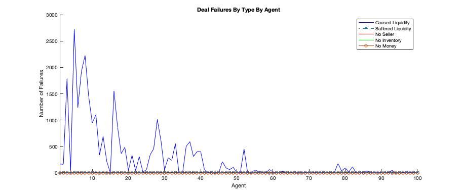
The following graphs plot transaction failure by agent and provide deeper insight into the model dynamics as a whole.
A further definition:
- Caused Liquidity Failure: An agent was on a proposed transaction path and invalidated the path due to a lack of liquidity. It does not imply the transaction failed ultimately failed as the next path analyzed may have been liquid (or the next, etc.). As you will see the total number of "caused" liquidity failure is typically much greater than the total "suffered" transaction failures.
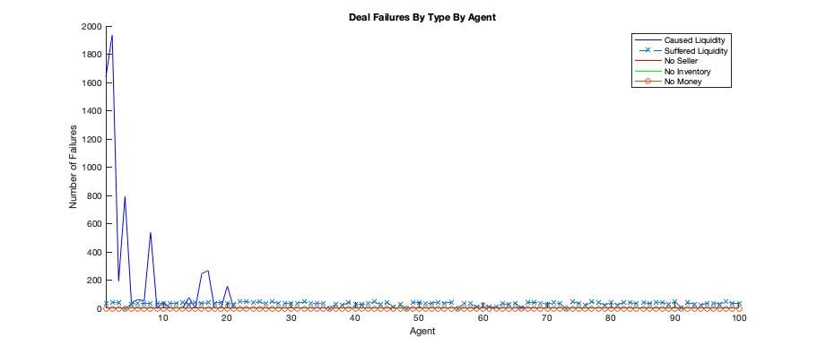
Simulation A1
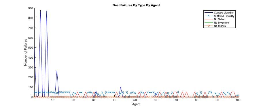
Simulation A1 - Iteration 1 Statistics (4940 possible transactions)
| Sales Efficincy | Successful Transactions | "Suffered" Liquidity Failures | "Caused" Liquidity Failures |
|---|---|---|---|
| 27% | 1,323 | 2,733 | 2,733 |
We can observe
- Most agents "suffered" liquidity failures evenly (aqua line)
- No Seller failures totaled 884 and tended to be bore by newer agents possessing fewer connections (to the right) (red line)
- The agents "causing" the vast majority of the liquidity failures are the oldest, most connected agents (to the left) (blue line)
- In this instance number of "caused" liquidity failures equals the number of "suffered" liquidity failures indicating (unexpectedly) that in this network there were no alternative paths between Buyer and Seller and it was either liquid or illiquid.
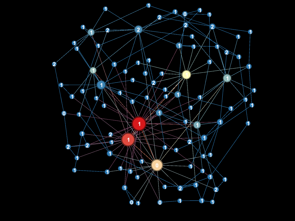
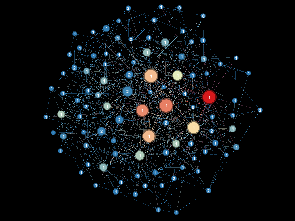
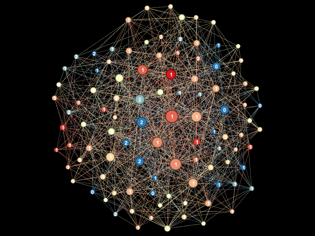
For a different perspective the following diagrams shows the network with the distribution of "caused" and "suffered" liquidity failures superimposed.
Note the size of the nodes are proportional to the nodes degree (number of connections), the node number is 1 if the node represents a Buyer, 2 if the node represents a Buyer / Seller and 0 for a Passive node.
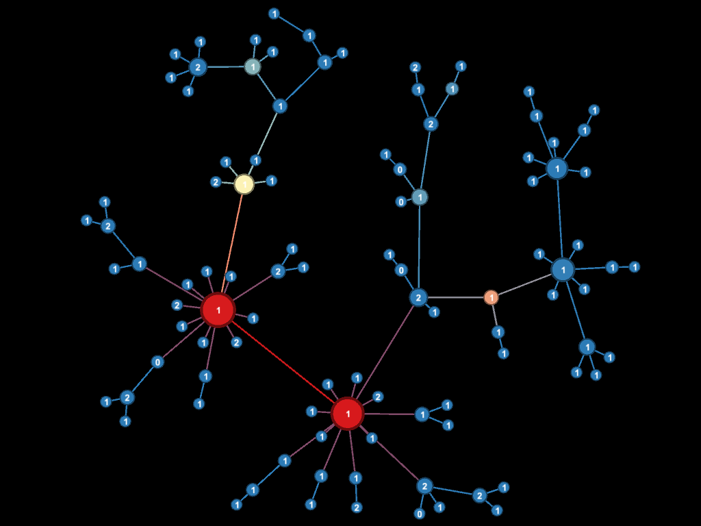
The "caused" liquidity failures are colored by a Blue-Yellow-Red spectrum with red depicting the greatest number of caused failures and blue depicting the least.
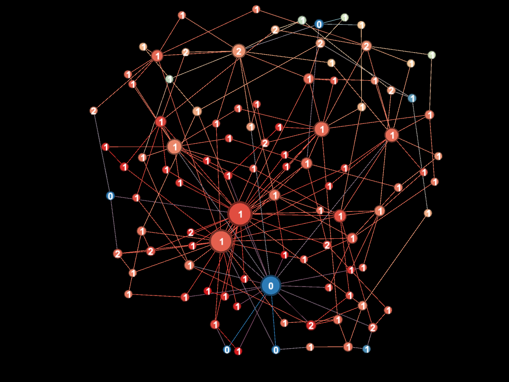
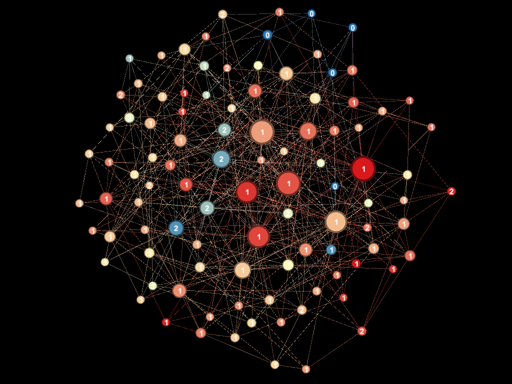
By contrast the following diagram shows the distribution of "suffered" liquidity failures.
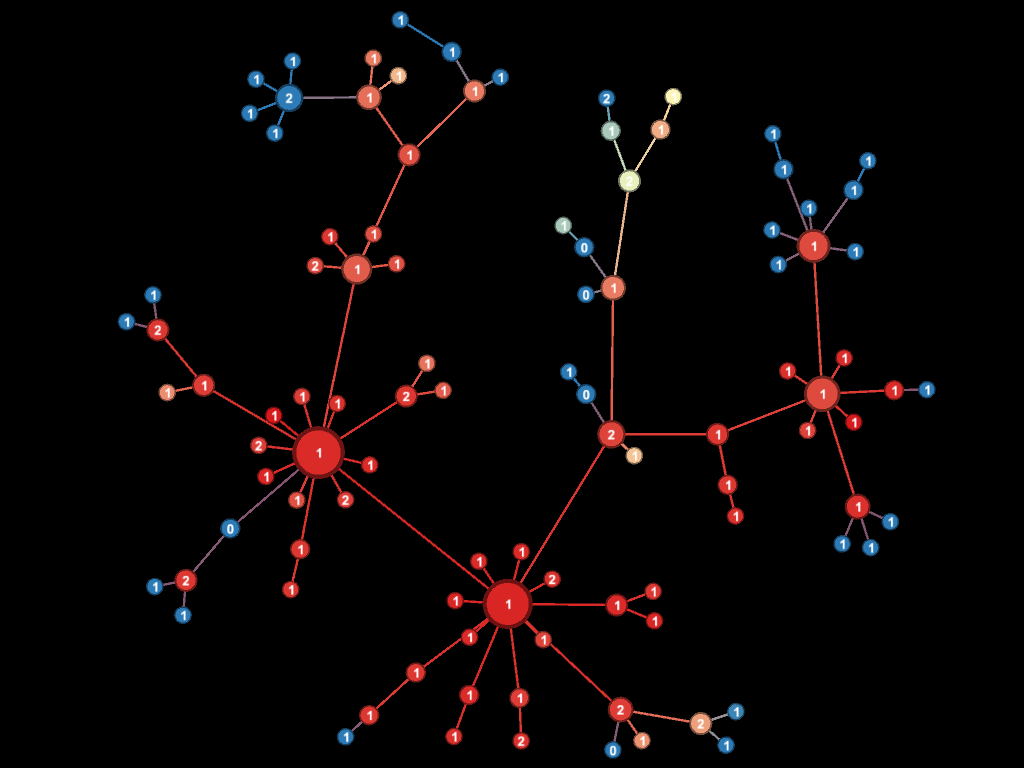
The "suffered" liquidity failures are colored by a Blue-Yellow-Red spectrum with red depicting the greatest number of suffered failures and blue depicting the least.
Finally we show the distribution of transaction failures by type in time (below). It shows that all the transaction failures occur more or less constantly in time and are not a result, for example, of the bootstrapping process or similar phenomenon.
For brevity we omit this last corresponding graph for the remaining models as they show the same constant behavior in time.
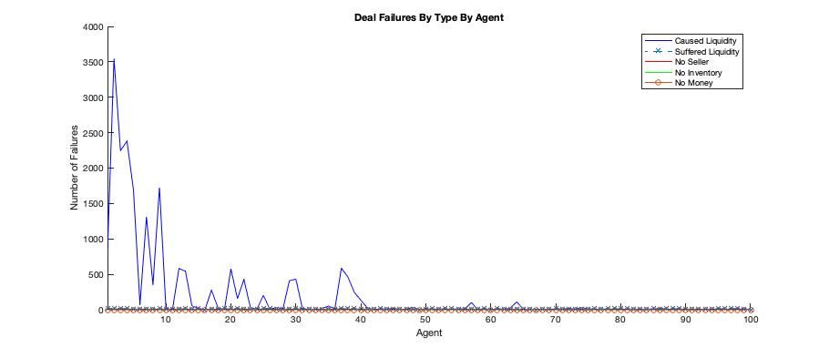
Simulation A2
Simulation A2 - Iteration 1 Statistics (4940 possible transactions)
| Sales Efficincy | Successful Transactions | "Suffered" Liquidity Failures | "Caused" Liquidity Failures |
|---|---|---|---|
| 34% | 1,671 | 3,269 | 6,083 |
We can observe
- Most agents "suffered" liquidity failures evenly
- The agents "causing" the vast majority of the liquidity failures are the oldest, most connected agents (to the left)
- The number of the "suffered" liquidity failures went up because the network configuration eliminated the no seller failures.
- The number of "caused" liquidity failures increased as well. We can interpret this to mean it took 6083 failures to find 1761 liquid paths or a ratio of ~3.6.
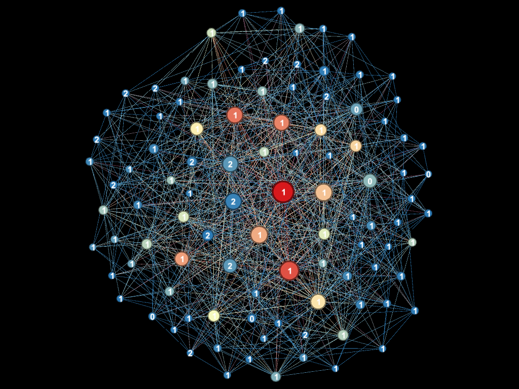
For comparison the network view of "caused" and "suffered" liquidity failures are provided below.
Simulation A3
Simulation A3 - Iteration 1 Statistics (4940 possible transactions)
| Sales Efficincy | Successful Transactions | "Suffered" Liquidity Failures | "Caused" Liquidity Failures |
|---|---|---|---|
| 79% | 3,891 | 1,049 | 20,023 |
We can observe
- "Suffered" liquidity failures dropped significantly as more deals (almost double) were completed successfully
- The agents causing the vast majority of the liquidity failures are the oldest, most connected agents (to the left), but the spectrum is moving out to the right, the burden is being shared
- The number of "caused" liquidity failures continue to increase. This is showing us that while the more dense network is indeed providing more opportunity to search for liquid paths (probably longer paths), there remain increasing many paths that are not liquid. Note the ratio of "caused" liquidity failures to "successful" transactions has risen to ~5x
For comparison the network view of "caused" and "suffered" liquidity failures are provided below.
Simulation A4
Simulation A4 - Iteration 1 Statistics (4940 possible transactions)
| Sales Efficincy | Successful Transactions | "Suffered" Failures | "Caused" Failures |
|---|---|---|---|
| 94% | 4,663 | 277 | 26,773 |
We can observe
- "Suffered" liquidity failures again dropped significantly as more deals were completed successfully
- The agents causing the vast majority of the liquidity failures are the oldest, most connected agents (to the left), but the spectrum continue to move further out to the right
- Again the number of "caused" liquidity failures rose, but not by as much, and they are more spread out across more agents. Note the ratio of "caused" liquidity failure to "successful" transactions has risen to ~5.7x. Since we have almost reached a sales efficiency of 100% we might view the value of ~6x to be an upper limit, at least for this network configuration.
For comparison the network view of "caused" and "suffered" liquidity failures are provided below.
It's clear from the network plots that we see a continued loosening of liquidity constraints as we move from Model 1 to 4.
Percentage Of Sellers
Another parameter that has a direct impact on the number of liquidity failures is the number of sellers that exist on the network.
More sellers mean more buying from trusted neighbors and less reliance on transitive-transactions to complete transactions. It also means more, potentially shorter, paths are available when searching for a liquid path.
Using the global model parameters presented above, in this simulation we vary the percentage of sellers using the network Model 2 - 4% density. The results are given in the table below.
| Simulation # | % Sellers | % Sales Efficency | % Liquidity Failure | % No Seller Failure |
|---|---|---|---|---|
| B1 | 5% | 20% | 78% | 2% |
| B2=A2** | 15% | 31% | 69% | 0% |
| B3 | 25% | 42% | 58% | 0% |
| B4 | 50% | 62% | 38% | 0% |
| B5 | 75% | 73% | 22% | 0% |
| B6 | 100% | 93% | 7% | 0% |
** Note Simulation B2 is the equivalent of A2 above
With Model 2 we need a very high percentage of sellers to achieve the target 90% for sales efficiency. Even with 100% Sellers (translating to 95 Buyer / Seller agents) the network still experiences significant Liquidity Failures.
We can glean two results from this simulation suite:
- The % of Sellers is not as strong an influence as is Network Density
- The combination of % of Sellers and Network Density can be a powerful combination to achieve high sales efficiency with smaller numbers of Sellers and less dense networks.
Future work will further delve into this space.
Price / UBI
The final option analyzed in depth was to load the system with enough money such that liquidity situations disappear.
In other words, if everybody has enough savings compared to what they are spending then they can always support a transitive transaction.
In this simulation we chose 5% Sellers and Model 2 - 4% density and varied the Price versus UBI.
| Simultion # | Price / UBI | % Sales Efficency | % Liquidity Failure | % No Seller Failure |
|---|---|---|---|---|
| C1 | 1% | 99% | 0% | 1% |
| C2 | 5% | 93% | 4% | 3% |
| C3 | 10% | 77% | 22% | 1% |
| C4 | 25% | 46% | 52% | 2% |
| C5 | 50% | 29% | 70% | 1% |
| C6=B1** | 90% | 20% | 78% | 2% |
** Note Simulation C6 is the equivalent of B1 above with UBI = 360 and the Price 324 (or 90% of the UBI)
Here we see a Price / UBI of approximately 5% or lower is required to reach our sales efficiency target.
To put that in perspective, for this scenario, that means if the price of a basket of goods is 1 the corresponding UBI needs to be 20. This seems unattractive on its own.
Future Considerations
The key results from this analysis are the following:
- The transitive-transaction process places a large liquidity burden on the system which is unfair and a disincentive to the agents participating if their transactions are often blocked as a result
- We show there are achievable system configurations that can reduce or eliminate the liquidity effects such that they become invisible (or nearly so) to the participants, at least in the long run (versus bootstrapping)
- Promoting network density and a rich market (sellers) are the keys to eliminating the "liquidity" situation
There are other avenues available to us as well that will be analyzed in future work. Our model is still primitive and will continue to modernize.
Briefly the are:
Advance The Economic Model: Advancing the buy / sell dynamics is a high priority next step for us and in doing so may well improve the liquidity situation. For example, fewer transactions per time period would lesson the burden transitive-transactions puts on the system. Also, introducing different products, at different prices, purchased at different periodicities may have the same effect (while introducing new, yet unanalyzed dynamics)
Find Another Seller: Currently Sellers are selected randomly from the pool of Sellers that lie within the Buyers transaction-distance. If the transaction fails for some reason the algorithm moves on, it does not try to find another Seller. Relaxing this constraint may have a positive effect on sales efficiency.
Different Network Characteristics: We have adopted a network generation model based on the preferential attachment model which assigns new attachments weighted to agents that are well connected (a "rich" get "richer" model seen in many social networks). A random network, for example, would exhibit a different network structure with few clusters and would therefore produce different commerce dynamics. We plan to study this over time.
Variable Transaction-Distance: The transaction-distance is currently fixed. We know that if the transaction-distance is proportional to the diameter of the underlying network it serves little additional purpose, but if it's less than the diameter it will lead to No Seller failures. In this situation, if we increase it, we can essentially make more sellers available to the overall market. If the variability was temporally, it could be important aid during system bootstrapping.
Developing rules for a variable transaction-distance based on transaction type could be influential as well.
Alter The Transitive-Transaction Algorithm: Currently we always select the first shortest liquid path found between a buyer and seller. We do not consider other, equal in length or longer paths. If, for example, we randomly selected from the pool of all liquid paths we suspect this will lesson the burden on highly connected agents currently carrying the brunt of the transitive coin transfers.
Injection Schemes: We have focused heavily on finding model settings whereby the liquidity situation takes care of itself without any form of external "intervention". We feel this remains the right direction, but especially during bootstrapping, it may be useful to develop an intervention strategy. We have no specific offerings at this moment.