
To date we have presented parametric modeling results focused on economic "efficiency" and battles with the "liquidity" situation using networks of varying characteristics. In this article we turn our attention to more macro economic features, namely, the relationship between Universal Basic Income (UBI), Demurrage, Price Levels and the Money Supply.
Briefly reviewing our model, UBI is awarded to every agent on the network at a set time interval and Demurrage is applied or collected from every agent at a set time interval (the time intervals can be different). All demurrage collected from the system is "destroyed", meaning there is no mechanism to reintroduce these monies. The UBI award and the Demurrage percentage is the same for each agent and does not vary in time.
Therefore, the Money Supply at time t > t = 0 is defined to be the sum of all UBI awarded to all agents through time t minus the sum of all Demurrage "collected and destroyed" from all agents through time t.
If you are unfamiliar with the definitions and motivations for our economic model, including UBI and Demurrage, please review our blog post located here
The Simulations
We present below the relationship over time of UBI, Demurrage and the Money supply through six simulations whereby we vary the percentage of demurrage for two different UBI amounts, one with UBI > Price and the other with UBI < Price.
Normally our simulations consist of 16 separate iterations each. In this case we ran 8 iterations in each simulation as they are enough for the purposes of this discussion. We also normally run our iterations for 52 time steps (1 year), but this time we extended them to 208 time steps (4 years).
The inputs to all six simulations are the following. Note our prior simulations typically specified a UBI grant of 360 and a Demurrage percentage of 5% - so this would be our "baseline". Here we will analyze Demurrage at 5%, 10% and 50% and UBI of 360 and 90.
| Parameter | Value | Description |
|---|---|---|
| Time Steps | 208 | Simulation duration = 208 weeks or 4 years |
| Total Agents | 100 | Total agents on network |
| Passive Agents | 5% | % agents do not buy or sell |
| Selling Agents | 15% | % agents that buy and sell |
| Price | 324 | The price of a basket of goods, ~90% of the UBI |
| Inventory | 3,000 | Initial inventory for each seller (essentially infinite) |
| Demurrage Interval | 4 | Demurrage is applied every 4 weeks |
| Demurrage Amount | 5% or 10% or 50% | Removed every 4 weeks |
| UBI Interval | 1 | UBI is granted each week |
| UBI Grant | 360 or 90 | 360 or 90 granted every week; no seed grant |
| Transaction-Distance | 3 | Maximum transaction distance on network |
| Iterations | 1 | A simulation consists of 1 model iterations |
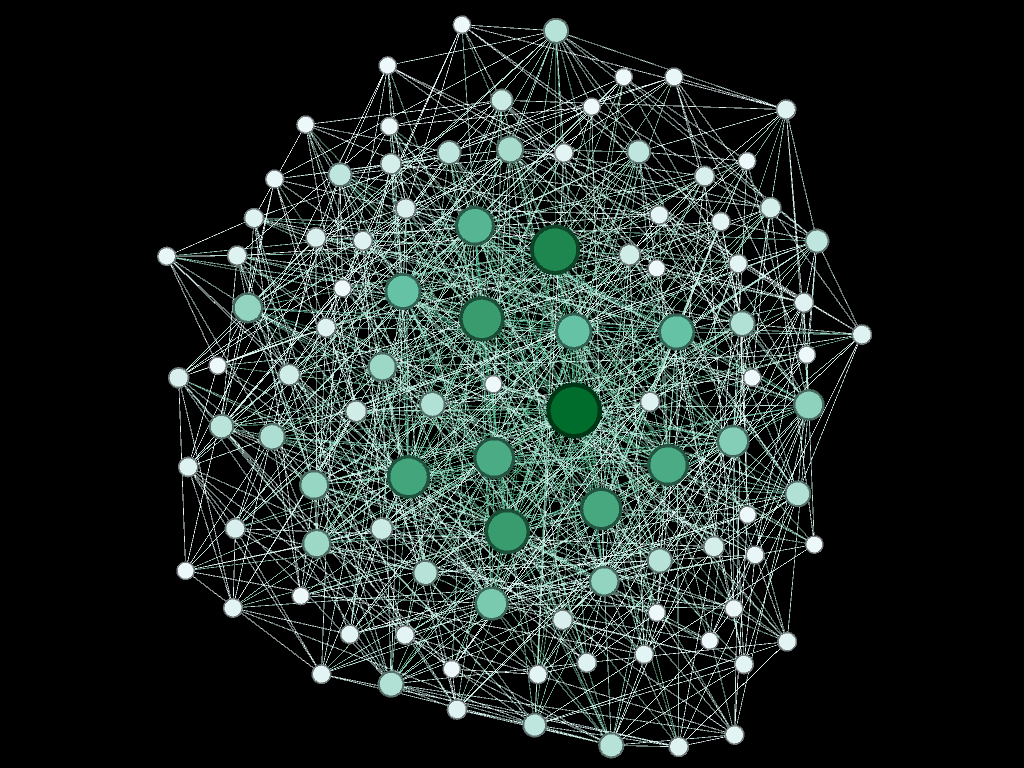
Additionally we employed our static network model M4 which consists of 100 agents and has a network density of 19%, diameter of 3 and average degree of 20. Previously discussed simulations using M4 showed it can be a highly liquid network.
You can learn more about our network models here. A picture of model M4 is provided below.
Some useful definitions are:
Sales Efficiency (SE): Sales Efficiency is the ratio of successfully completed transactions divided by the total possible transactions that could occur in a given model iteration. We seek scenarios where the aggregated SE >= 90%. The results below correspond to the mean value for all iterations in a simulation unless othewise stated.
Suffered Liquidity Failures (SLF): If a transaction fails due to a lack of liquidity on all available paths between a Buyer and Seller we call that a "Suffered" Liquidity Failure ("suffered" by the Buyer).
No Money Failure (NMF): If it's time for a Buyer to make a purchase and they do not have enough of the right combination of coins to meet the purchase price no transaction takes place and we call this a No Money Failure.
Caused Liquidity Failure (CLF): An agent on a possible transaction path invalidated the path due to a lack of liquidity. Such a failure does not imply the transaction ultimately failed as all possible paths are tested until a liquid one is found or the list is exhausted. If follows then that the total number of "Caused" liquidity failures is typically much greater than the total "Suffered" transaction failures.
The results of the simulations are provided below.
| Sim. | UBI | Demurrage | % SE | % SLF | % NMF |
|---|---|---|---|---|---|
| 1 | 360 | 5.0% | 91% | 9% | 0% |
| 2 | 360 | 10.0% | 94% | 6% | 0% |
| 3 | 360 | 50.0% | 86% | 14% | 0% |
| 4 | 90 | 5.0% | 30% | 53% | 17% |
| 5 | 90 | 10.0% | 30% | 41% | 29% |
| 6 | 90 | 50.0% | 24% | 29% | 47% |
First we observe that with a UBI grant of 360, which is greater than the purchase price of the basket of goods of 324, different percentages of demurrage do not have a large effect on Sales Efficency. In fact it takes 50% Demurrage to start to see a real dent in Sales Efficiency. The system is fairly liquid and we see no No Money Failures, just "Suffered" Liquidity Failures.
Quartering the UBI to 90 (Price >> UBI award), however, definitely starves the system of liquidity for all percentages of Demurrage and we see a corresponding large increase in "Suffered" Liquidity Failures and "No Money" Failures. We'll return to the interplay of these two failure types a bit later.
UBI, Demurrage and the Money Supply
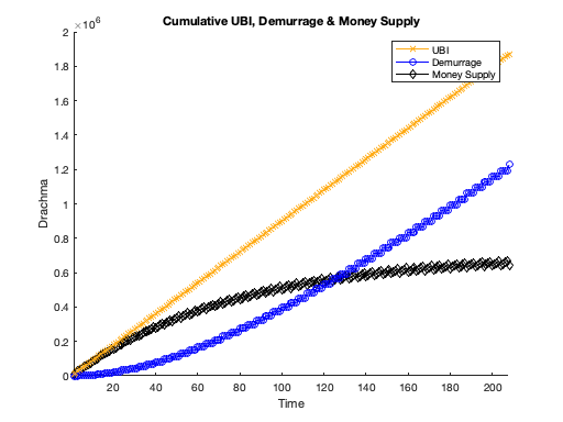
The graphs below plot cumulative UBI, Demurrage and the Money supply over time. The graph corresponding to Simulation 1, Iteration 1 is shown below.
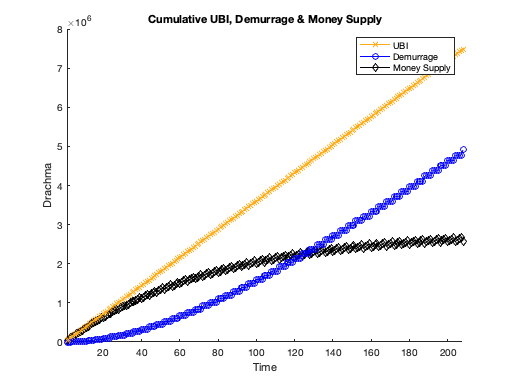
Overall we see total UBI accumulating at a constant rate. Cumulative demurrage rises slowly but eventually assumes an accumulation rate equal to the UBI accumulation rate. The money supply grows rapidly, slows and then asymptotically approaches a constant value (tracking as the inverse of cumulative demurrage).
In the case of 5% demurrage (above) we see the money supply and the cumulative demurrage crossing about ~120 weeks (~2.3 years), with the money supply seeming to be leveling off at ~2.6m units.

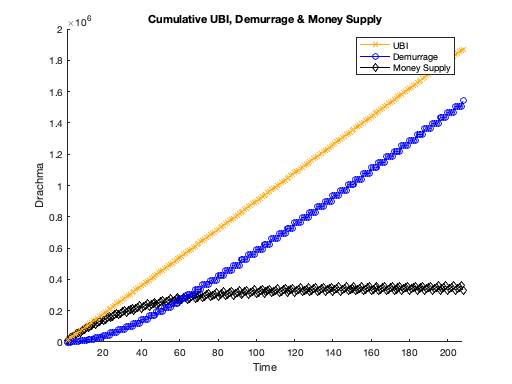
In the case of 10% demurrage (above) the money supply and cumulative demurrage cross at approximately 60 weeks (about half ot 5% demurrage) with the money supply leveling off at ~1.3M units of currency. Otherwise the relationships appear the same to the 5% demurrage example.
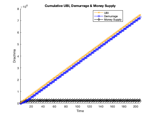
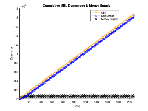
Finally in the extreme case of 50% demurrage we see the money supply and the cumulative demurrage crossing at ~10 weeks with the money supply leveling off at about ~0.18M units.
In summary, barring other shocks, we observe that smaller percentages of demurrage lengthen the time it takes to bring the money supply to its equilibrium while larger percentages of demurrage shorten the timing of stabilization of the money supply.
In fact, if UBI and Demurrage are applied at the same time interval, a halving of the percentage demurrage will double the timing and level of the equilibrium money supply and visa versa.
Now lets look at the same graphs for UBI = 90.
In the case of UBI = 90 and Demurrage = 5% (above) we observe the same cross over timing of the money supply and demurrage as simulation 1 of ~120 time steps, but the level of the equilibrium money supply is ~0.65M instead of ~2.6M (a quarter).
Similarly in the case of UBI = 90 and Demurrage = 10% (above) we observe the same cross over timing of the money supply and demurrage as simulation 2 of ~60 time steps, with the level of the equilibrium money supply is ~0.3M instead of ~1.3M.
Finally in the case of UBI = 90 and Demurrage = 50% (above) we observe the same cross over timing of the money supply and demurrage as simulation 3 of ~10 time steps, with the level of the equilibrium money supply is ~0.05M instead of ~0.18M.
At this point we have shown Demurrage controls the time that the money supply can grow while UBI sets the rate of money accumulation until equilibrium is reached.
Money Supply By Agent
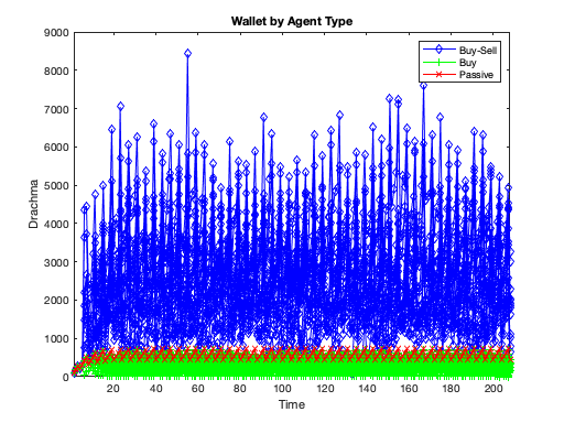
Continuing, let's look at a depiction of the money each agent possesses over time. We have three agent types: Buy and Sell agents, Buy-only agents and Passive agents (those that do not participate at all). The graphs for simulations 1-3 are provided below.
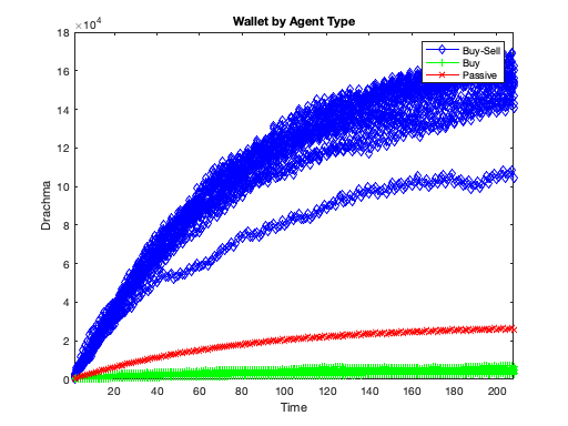
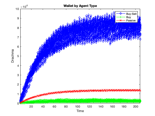
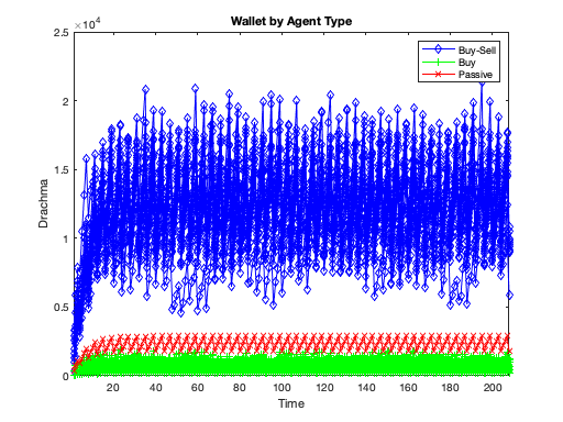
The figures above show the amount of total currency in each agents wallet over time (100 agents). We see that Buy-Sell agents collect the vast majority of the money (because they are selling) while the Buy-only agents retain the least amount of money (because they are only buying). Passive agents appear to build money in an analogous rate to the overall money supply.
It's interesting to note that the Buy-Sell agents are "penalized" most heavily by demurrage, since they carry the biggest balances, even though they represent the economic "makers". Also interesting is the "chatter" observed in the 50% Demurrage example where we can easily see the huge chunks of money being removed from the system periodically (every 4 weeks).
For completeness below we plot the corresponding graphs for the UBI = 90 scenarios 4-6 below.
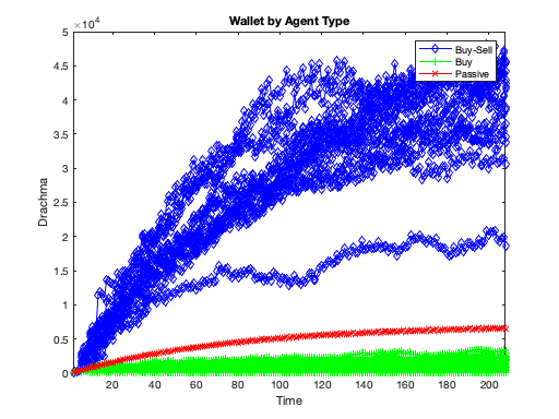
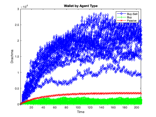
We again note the equilibrium amount in each wallet is lower because the money supply is lower (compared to the UBI =360 examples). Otherwise, we can confirm we see the same overall patterns.
Observations
The simulations presented do a good job of showing the basic relationships between UBI, Demurrage and the Money Supply over time.
We observed:
- Due to Demurrage the Money Supply (and average wallet size by agent type) equilibrates after a bootstrapping period
- The time to reach the money supply maximum or equilibrium is controlled by the Demurrage percentage
- The rate of growth of the money supply until equilibrium is controlled by the UBI award
- Combined, Demurrage and UBI determine the ultimate level of the money supply
- If the UBI is greater than the price of a basket of goods, modest percentages of Demurrage have little effect on the overall economic efficiency. No Money Failures do not occur as there is ample money to meet the sales price and achieve high levels of sales efficiency. As long as UBI > Price, these general results would hold regardless of the absolute UBI grant.
- If the UBI is less than the price of a basket of goods, the overall economic efficiency suffers significantly at all Demurrage percentages and an interplay between No Money Failures and Suffered Liqidity Failures occurs (the system is starved of liquidity to both make purchases and support transitive-transactions). As long as UBI < Price, these general results would hold regardless of the absolute UBI grant.
- The Money Supply and Sales Efficiency are loosely related. There needs to be enough money in the system such that liquidity failures are (nearly) eliminated (Suffered and Caused) which allows high levels of sales efficiency to be achieved. And the controlling knobs are the UBI award, the Demurrage percentage and interestingly, with respect to Sales Efficiency, the Price of the basket of goods.
Up until now, our model has not directly considered savings scenarios, as the UBI grant has always been greater than the price of a basket of goods (we purposely did this to not induce No Money Failures so we could study other parameters unmasked).
In this analysis we uncovered the "savings" situation in an effort to severely starve the system of liquidity to observe what would happen. To do this we lowered the UBI award to much less than the price of the basket of goods.
In other words, UBI grants less than the price of a basket of goods forces saving between successive buying opportunities, mostly for Buyer-only agents. Buyer-Sellers will generally quickly earn enough money to not suffer No Money Failures when they buy.
It could be argued that in the presence of No Money Failures our definition of Sales Efficiency may need revisiting as it currently tabulates being out of money as a missed commerce opportunity.
The "Savings" Situation
Further analysis into the "savings" situation is required, but before we depart, we can can use the six simulations presented in this article to dig a bit deeper into the dynamics for when the UBI award is less than the Price of goods.
The following three graphs display Deal Failures By Type, In Time for simulations 1-3, which are the cases when the UBI award is greater than the Price of goods.
We see for all three simulations the only failure is "Suffered" Liquidity Failures and the average number of failures in time is more or less constant at all levels of Demurrage after a small, transient bootstrapping period. Statistically we see no difference between the 5% and 10% Demurrage scenarios. The average number of failures increases by about 33% for the 50% Demurrage case. And given the associated high levels of sales efficiencies associated with each scenario we know the number of failures is small compared to the number of successful transactions.
Next we show the same three graphs for the UBI = 90 scenarios 4-6.
In these graphs we see the emergence of the No Money Failures due to "forced" savings. Again, after a bootstrapping period the No Money Failures and "Suffered" Liquidity Failures reach an equilibrium in time. For the 5% and 10% Demurrage cases Liquidity failures dominate the No Money failures. For the 50% Demurrage case the situation is reversed with No Money failures dominating the Liquidity failures.
What's most noteworthy is for the UBI < Price scenarios we see a resurgence of the Liquidity situation in the form of a consistent lack of liquidity for transitive-transactions even when the purchase price can be met and on networks we know are very liquid in UBI > Price scenarios.
To reinforce this observation, lets redefine Sales Efficiency to exclude No Money Failures from its calculus. Recalculating the simulation results from above in the table below we can clearly see the cost of forced savings in terms of the impact it has on liquidity for purchases and as a result Sales Efficiency.
| Sim. | UBI | Demurrage | % SE | % SLF | % NMF |
|---|---|---|---|---|---|
| 1 | 360 | 5.0% | 91% | 9% | 0% |
| 2 | 360 | 10.0% | 94% | 6% | 0% |
| 3 | 360 | 50.0% | 86% | 14% | 0% |
| 4 | 90 | 5.0% | 36% | 64% | 0% |
| 5 | 90 | 10.0% | 43% | 57% | 0% |
| 6 | 90 | 50.0% | 45% | 55% | 0% |
Bottom line, the liquid network with UBI > Price is quite illiquid with UBI < Price.
A final note would be that the equilibrium levels of liquidity failure and no money failure in all simulations is reached at a time seemingly independent from the accumulation and equilibrium timing of the money supply.
Summary
We have presented the relationships graphically and otherwise between UBI, Demurrage and the Money Supply. We observed the money supply is controlled by both the UBI award and the Demurrage percentage. Demurrage controls how long it takes the money supply to equilibrate and the UBI award sets the rate of accumulation until equilibrium is reached. We also saw that the long term money supply is a proxy or mirror to long term sales efficiency.
We also uncovered the "savings" situation whereby when UBI < Price a liquid network with UBI > Price can become illiquid from a transitive-transaction viewpoint, which stymies the economic efficiency.
Future work will look deeper into the "savings" situation and the relationship between the long term level of the money supply and sales efficiency. It's worth saying that the UBI < Price situation may turn out to not be very common.
We now have presented most of our key results regarding our V1.0 economic model, namely, Model Dynamics and the "Liquidity" Situation, Model Dynamics for different Networks and now this article discussing UBI, Demurrage and the Money Supply. Next we will turn towards advancing the economic model to include different types of buyers and sellers and thereby take a next step towards modeling a complex commerce situation.