
Our first economic analysis presented results from simulations using four static networks of varying statistical qualities each having 100 agents. In this post we present results that extend the analysis by using static networks possessing similar statistical qualities but each having 1000 agents.
What we found is the larger, less dense networks are more liquid than their smaller, more dense counterparts.
In review, to date we have focused on studying commerce over a trust-based social network whose transactions are governed by a transitive-transaction model. The main inhibitor to commerce has been what we playfully call the "liquidity situation" whereby transactions fail due to insufficient liquidity to support the desired transitive-transactions. This study continues our research into the dynamics of our model and the search for ways reduce or eliminate liquidity issues.
For reference, you can find our prior (first) model dynamics analysis here. If you are unfamiliar with the specifics of our economic model please read about it here. Further details regarding the transitive-transaction algorithm itself may be found here, while the "liquidity situation" is discussed here.
The table below lists the global input parameters used in each simulation presented in this article. These are the same as were used in our prior analysis with very slight modification.
| Parameter | Value | Description |
|---|---|---|
| Time Steps | 52 | Simulation duration = 52 Weeks |
| Total Agents | 100 or 100 | Total agents on network |
| Passive Agents | 5% | % agents do not buy or sell |
| Selling Agents | 15% | % agents that buy and sell |
| Price | 300 | The price of a basket of goods, ~80% of the UBI |
| Inventory | 3,000 | Initial inventory for each seller (essentially infinite) |
| Demurrage Interval | 4 | Demurrage is applied every 4 weeks |
| Demurrage Amount | 5% | 5% removed every 4 weeks (60% annually) |
| UBI Interval | 1 | UBI is granted each week |
| UBI Grant | 360 | 360 granted every week; no seed grant, 1,400 monthly |
| Transaction-Distance | 3 | Maximum transaction distance on network |
| Iterations | 16 | A simulation consists of 16 model iterations |
Some useful definitions are:
Simulation: One execution of the model is named an iteration. A simulation consists of the aggregated results from all iterations, 16 in our case here (because my computer has 8 cores and we can parallelize 8 iterations at a time).
Sales Efficiency (SE): Sales Efficiency is the ratio of successfully completed transactions divided by the total possible transactions that could occur in a given model iteration. We seek scenarios where the aggregated SE >= 90%. The results below correspond to the mean value for all iterations in a simulation unless othewise stated.
Suffered Liquidity Failures (SLF): If a transaction fails due to a lack of liquidity on all available paths between a Buyer and Seller we call that a "Suffered" Liquidity Failure ("suffered" by the Buyer).
No Seller Failure (NSF): If it's time for a Buyer to make a purchase and there exists no Sellers on the network within the transaction-distance of the Buyer we call that a No Seller Failure.
Caused Liquidity Failure (CLF): An agent on a possible transaction path invalidated the path due to a lack of liquidity. Such a failure does not imply the transaction ultimately failed as all possible paths are tested until a liquid one is found or the list is exhausted. If follows then that the total number of "Caused" liquidity failures is typically much greater than the total "Suffered" transaction failures.
Network Density
Previously we presented simulation results A1-4 for the economic scenario described above using our static network models M1-4, each possessing 100 agents. Here we present and compare new simulation results A5-8 employing the same economic scenario and using our network models M5-8, each possessing 1000 agents.
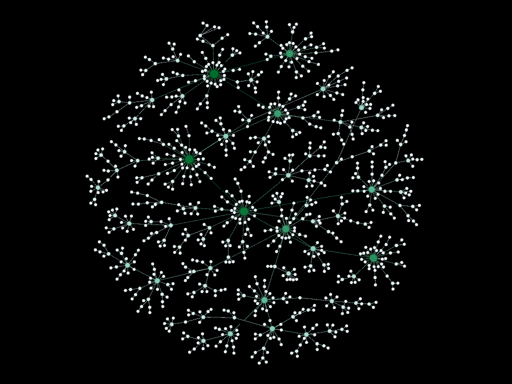
A detailed description of the network models M1-8 and how they were generated using a preferential attachment model can be found here.
We represent the key network statistics for all models M1-8 in the table below, slightly rearranged by grouping the like networks. Each group used the same network generation process and stopped at either 100 or 1000 agents.
| Model | Agents | Avg. Degree | Diameter | Density | Clustering Coef. |
|---|---|---|---|---|---|
| M1 | 100 | 2 | 12 | 2% | 0.0 |
| M5 | 1000 | 2 | 19 | 0.05% | 0.0 |
| M2 | 100 | 4 | 6 | 4% | 0.17 |
| M6 | 1000 | 4 | 7 | 0.8% | 0.03 |
| M3 | 100 | 10 | 3 | 10% | 0.22 |
| M7 | 1000 | 10 | 5 | 1% | 0.05 |
| M4 | 100 | 19 | 3 | 20% | 0.35 |
| M8 | 1000 | 20 | 4 | 2% | 0.07 |
From a statistical perspective, each of the 4 groups have similar network Degree and Density topologies with the 1000 agent networks M5-8 being much less dense and have lower levels of clustering than the 100 agent networks M1-4.
Results and Further Comparisons
Sales Efficiency and Network Density
We present below the results of the prior simulations A1-4 and the new simulations A5-8, grouped as we did above with the network statistics.
| Simulation | Agents | Model/Density | % SE | % SLF | % NSF |
|---|---|---|---|---|---|
| A1 | 100 | M1 / 2% | 23% | 62% | 15% |
| A5 | 1000 | M5 / 0.05% | 18% | 72% | 10% |
| A2 | 100 | M2 / 4% | 31% | 69% | 0% |
| A6 | 1000 | M6 / 0.80% | 25% | 75% | 0% |
| A3 | 100 | M3 / 10% | 71% | 29% | 0% |
| A7 | 1000 | M7 / 1% | 42% | 58% | 0% |
| A4 | 100 | M4 / 19% | 94% | 6% | 0% |
| A8 | 1000 | M8 / 2% | 73% | 27% | 0% |
We observe
- The 1000 agent networks M5-8 fare less well than their M1-4 counterparts in terms of sales efficiency (SE) and sales failures (SLF and NSF). This is expected since we learned in the A1-4 experiment that increased network density reduces liquidity failures and increases sales efficiency
- However a closer look shows models M5-8 with 1000 agents actually perform better when noting they reach higher levels of sales efficiency at lower levels of model density
If we plot the results this observation becomes more clear (below).
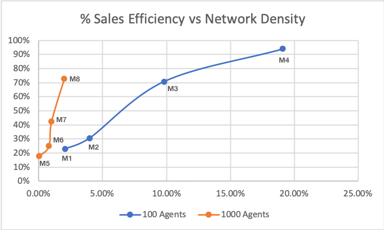
A key result of this comparison is, all things being equal, larger, less dense networks can be much more liquid than smaller, more dense networks.
In fact here it looks like the 1000 agent networks project to reach 100% sales efficiency at ~< 5% while the 100 agent networks project to reach that level at ~> 20%. This is noteworthy because it means high levels of liquidity for transitive-transactions can be achieved with networks that are not very dense or clustered.
Sales Efficiency And Liquidity Failures
The table below shows more of the simulation details. We do not (yet) have aggregated values for all these data and so the numbers below correspond to the first iteration of each simulation (which is sufficient for this discussion).
| Simulation | SE | Possible Trans. | Successful Trans. | SLF | CLF | CLF/Successful |
|---|---|---|---|---|---|---|
| A1 | 27% | 4,940 | 1,323 | 2,733 | 2,733 | 2 |
| A5 | 18% | 49,440 | 8,954 | 35,870 | 35,870 | 4 |
| A2 | 34% | 4,940 | 1,671 | 3,269 | 6,083 | 4 |
| A6 | 22% | 49,440 | 10,896 | 38,452 | 45,309 | 4 |
| A3 | 79% | 4,940 | 3,891 | 1,049 | 20,023 | 5 |
| A7 | 42% | 49,440 | 20,783 | 28,617 | 122,356 | 6 |
| A4 | 94% | 4,940 | 4,663 | 227 | 26,773 | 6 |
| A8 | 71% | 49,440 | 35,013 | 14,385 | 474,606 | 14 |
We observe
- For simulations A1 and A5 the Suffered (SLF) and Caused failures (CLF) are the same indicating that this network group M1 and M5 is binary in liquid paths; either a liquid path is available or it's not, there are no alternative paths
- For all simulations A1-A8 the Caused failures are greater than the number of successful transactions, increasingly so as the network density increases.
- Simulation A8 analyzed 474,606 failed paths and 34,013 successful paths for a total of 508,619 paths in one iteration!
Remember the Caused failures represent the number of paths searched that failed due to a lack of liquidity on the way to finding the liquid paths that completed the sales successfully.
Looking deeper, the figure below plots sales efficiency versus the ratio of failed to successfully searched paths ("Caused" to Successful Transactions or CLF / Successful).
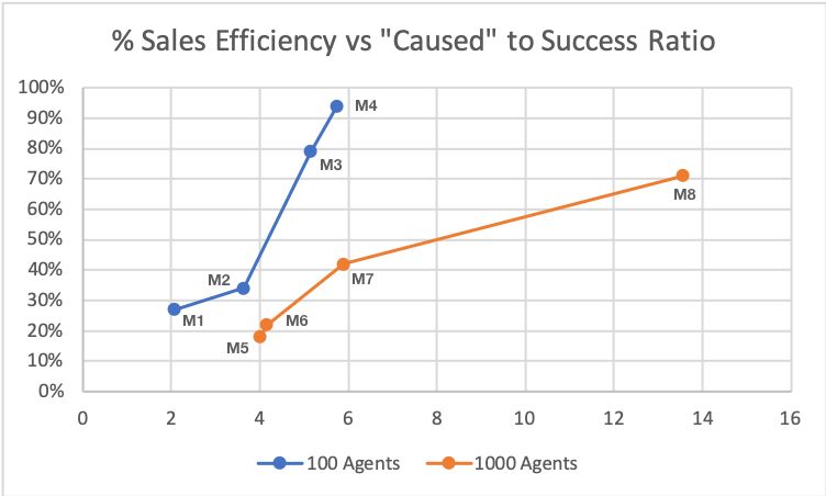
We observe
- The 100 agent networks M1-4 have a fail / success ratio of ~2 to ~6. Since M4 possesses a sales efficiency of > 90% we can be sure the fail / success ratio is near its maximum
- The 1000 agent networks M5-8 have a fail / success ratio of ~4 to ~14. Given simulation A8 has a sales efficiency of ~70% we can expect the fail / success ratio to climb quite a bit higher on the way to 100% sales efficiency
Therefore, we can conclude that while the M5-8 networks are more liquid from a transitive-transaction perspective than their M1-4 counterparts, comparatively many more failed paths are being evaluated along the way (a factor of maybe 20 versus 6).
This said we can expect more dense 1000 agent networks to perform better while requiring proportionately fewer paths.
Summary
The key results from the prior analysis were:
- The transitive-transaction process places a large liquidity burden on the system which is unfair and a disincentive to the agents participating if their transactions are often blocked as a result
- We showed there were achievable system configurations that can reduce or eliminate the liquidity effects such that they become invisible (or nearly so) to the participants, at least in the long run (versus bootstrapping)
- Promoting network density and a rich market (numerous sellers) are the keys to eliminating the "liquidity" situation in a natural way
These conclusions remain true and now we can add:
- A additional lever to managing the "liquidity" situation is to increase the size of the network as larger networks are more liquid, even at very low network densities.
- The computational effort employed to search for all the liquid paths may make scaling to larger networks a challenge. For example, simulation A8 required ~73 hours computation time per iteration on a powerful laptop computer (with 8 iterations running in parallel). This will be another necessary area of further research.